from fastai2.vision.all import *
from fast_impl.core import get_module, arch_summary, min_max_scale
path = untar_data(URLs.IMAGEWOOF_320)
lbl_dict = dict(
  n02086240= 'Shih-Tzu',
  n02087394= 'Rhodesian ridgeback',
  n02088364= 'Beagle',
  n02089973= 'English foxhound',
  n02093754= 'Australian terrier',
  n02096294= 'Border terrier',
  n02099601= 'Golden retriever',
  n02105641= 'Old English sheepdog',
  n02111889= 'Samoyed',
  n02115641= 'Dingo'
)
dblock = DataBlock(blocks=(ImageBlock,CategoryBlock),
                   get_items=get_image_files,
                   splitter=GrandparentSplitter(valid_name='val'),
                   get_y=Pipeline([parent_label,lbl_dict.__getitem__]),
                   item_tfms=Resize(320),
                   batch_tfms=[*aug_transforms(size=224),Normalize.from_stats(*imagenet_stats)])
dls = dblock.dataloaders(path,bs=128)
dls.show_batch()

exp_name='resnet34'
save_model = SaveModelCallback(monitor='error_rate',fname=exp_name)
body = create_body(resnet34,cut=-2);
nf = num_features_model(body)
head = nn.Sequential(nn.AdaptiveAvgPool2d((1,1)),Flatten(),nn.Linear(nf,dls.c))
model = nn.Sequential(body,head)
def resnet_split(m): return L(m[0][:6], m[0][6:], m[1:]).map(params)
learn= Learner(dls,model,metrics=error_rate,cbs=save_model,
               opt_func=ranger,splitter=resnet_split,
               model_dir='/content/models')
learn.fit_flat_cos(5,lr=1e-3)
learn.unfreeze()
learn.fit_flat_cos(4,lr=1e-4)
b = learn.dls.one_batch()
learn.dls.show_batch(b)

Same as above, but here to clarify the fact that we'll be working with the same image when indexed into batch for CAM/GradCAM
idx=5
x,y = b[0][idx],b[1][idx]
x,y = learn.dls.decode_batch((x[None],y[None]))[0]
show_image(x,title=y);

xb,yb = b[0][idx][None],b[1][idx][None]
Class Activation Mappping
CAM highlights the class specific desciminative region by mapping predicted class score to previous convolutional layer.
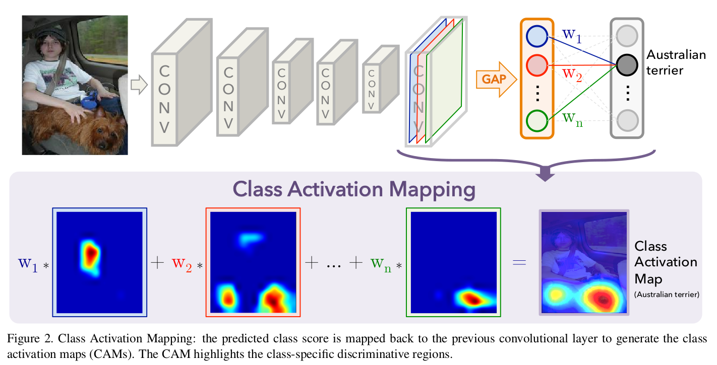
Here $M_c$ defines CAM for class C, $w_c^k$ is the weight corresponding to class c for unit k. $f_k(x,y)$ represent the activation of unit k in the last convolutional layer at spatial location (x,y)
m = learn.model
We want the output of penultimate layer from encoder part as last layer of it is Average Pool. Thus, we'll index that layer as m[0][-2].
hook = hook_output(m[0])
with torch.no_grad(): output = m.eval()(xb)
We know the label, let's check whether the model got it right
learn.dls.vocab[ output.argmax().item()]
Weights of Linear layer
wt = learn.model[1][-1].weight; wt.shape
Activation maps
act = hook.stored[0]; act.shape
We want to multiply a matrix with 3D tensor, in this case, a matrix of shape 10 x 512 and a Tensor of 512,7,7. We can do this by defining our custom matrix multiplication using torch.einsum
cam = torch.einsum('ck,kij->cij',wt,act).sum(0); cam.shape
sz = xb.shape[-1]; sz
def show_heatmap(x,cam,sz,merge=False,figsize=(7,7),
                 alpha=0.6,interpolation='spline36',
                 cmap='magma'):
  "Used to show CAM/gradcam"
  if merge: figsize=(4,4)
  if not merge: alpha=1.
  _,axs = subplots(1,1 if merge else 2,figsize=figsize)
  if not isinstance(x,TensorImage): x = TensorImage(x)
  x.show(ax=axs[0],title='Image' if not merge else None)
  if cam.dim()==2: cam = cam[None]
  show_image(min_max_scale(cam),ax=axs[0 if merge else 1],
             extent=(1,sz,sz,1),alpha=alpha,
             interpolation=interpolation,cmap=cmap,
             title='Heatmap' if not merge else None);
show_heatmap(x,cam,224,merge=True)

show_heatmap(x,cam,224)

m = learn.model
xb,yb = dls.one_batch()
The batch size is 128, so any idx in [0,127] is valid for the following snippet. We can specify max_n to show that many images.
dls.show_batch((xb,yb),ncols=5,max_n=20)

idx=15
xb,yb = xb[idx][None],yb[idx][None]
x_dec,y_dec = learn.dls.decode_batch((xb,yb))[0]
with hook_output(m[0]) as hook:
  y_pred = m.eval()(xb)
  pred_cls = dls.vocab[y_pred.argmax().item()]
  print(f"{'Actual':<9}: {y_dec}\nPredicted: {pred_cls}")
  act = hook.stored[0]
  cam = torch.einsum('ck,kij->cij', m[1][-1].weight, act).sum(0)
  show_heatmap(x_dec,cam,sz=x.shape[-1])

url = 'https://t2conline.com/wp-content/uploads/2020/01/shutterstock_1124417876.jpg'
fname = 'test-shih-tzu.jpg'
download_url(url,dest=fname)
img = PILImage.create(fname); img.show(figsize=(5,5))

Fastai2's test_dl applies your validation transforms to given image. So you need to exhibit all the type_tfms before passing an item to dataloader. You can find them as follows:
dls.tfms
We've created PILImage as per the pipeline and need a bit of extra work for label
xb, = first(dls.test_dl([img]))
y_lbl = dls.vocab[-1]; y_lbl
yb = dls.categorize(y_lbl)[None]; yb
Putting it in a handy function
def create_batch(fname,lbl_idx):
  """Create test_batch from filename and label index
  Refer `dls.vocab` to find validation index
  """
  x = PILImage.create(fname)
  xb, = first(dls.test_dl([img]))
  yb = dls.categorize(dls.vocab[-1])[None]
  return xb,yb
xb,yb = create_batch(fname,9)
def show_cam(learn,xb,yb,act_path:list=[0], wt_path:list=[1,-1],merge=True):
  """Show CAM for a given image
  `act_path`: list of indices to reach activation map layer
  `wt_path`: list of indices to reach weight layer
  `merge`: to use same axis for image and mask
  """
  m,dls = learn.model,learn.dls
  act_layer = get_module(model,act_path)
  wt_layer = get_module(model,wt_path)
  # pdb.set_trace()
  with hook_output(act_layer) as hook:
    y_pred = m.eval()(xb)
    pred_cls = dls.vocab[y_pred.argmax().item()]
    act = hook.stored[0]
    # pdb.set_trace()
    cam = torch.einsum('ck,kij->cij', wt_layer.weight, act).sum(0)

    x_dec,y_dec = dls.decode_batch((xb,yb))[0]
    print(f"{'Actual':<9}: {ifnone(y_dec,'')}\nPredicted: {pred_cls}")
    show_heatmap(x_dec,cam,sz=x.shape[-1])
We need to specify path to the activation layer and weigtht layer. It could be identified using arch_summary
arch_summary(learn.model,verbose=True)
For the activation layer, we can take the output of $0^{th}$ Sequential layer, which essentially is the encoder part of model. "Weight layer" is simply last layer of the model, which can be reached using [1,-1]
show_cam(learn,xb,yb,[0],[1,-1])
