from fastai2.vision.models.xresnet import *
from torchvision.models import resnet50
from fast_impl.core import *

arch_summary function plays major role while deciding parameter groups for discriminative learning rates. It gives a brief summary of architecture and is independant of input being passed. Thus we could use this function to understand architecture in a glance. We'll briefly explore various vision models from torchvision and pytorch-image-models to understand the use of arch_summary

XResNet (fastai2)

Let's first quickly go through XResNet series offered by fastai2

def xresnet18 (pretrained=False, **kwargs): return _xresnet(pretrained, 1, [2, 2,  2, 2], **kwargs)
arch_summary(xresnet18)
[0 ] ConvLayer        : 3   layers
[1 ] ConvLayer        : 3   layers
[2 ] ConvLayer        : 3   layers
[3 ] MaxPool2d        : 1   layers
[4 ] Sequential       : 2   layers
[5 ] Sequential       : 2   layers
[6 ] Sequential       : 2   layers
[7 ] Sequential       : 2   layers
[8 ] AdaptiveAvgPool2d: 1   layers
[9 ] Flatten          : 1   layers
[10] Dropout          : 1   layers
[11] Linear           : 1   layers

Look at the Sequential layers from 4-7 all having two child layers, that's the meaning of [2,2,2,2] in the model definition. Let's go deeper and check what are these two children

arch_summary(xresnet18,verbose=True)
[0 ] ConvLayer        : 3   layers
      Conv2d
      BatchNorm2d
      ReLU
[1 ] ConvLayer        : 3   layers
      Conv2d
      BatchNorm2d
      ReLU
[2 ] ConvLayer        : 3   layers
      Conv2d
      BatchNorm2d
      ReLU
[3 ] MaxPool2d        : 1   layers
[4 ] Sequential       : 2   layers
      ResBlock
      ResBlock
[5 ] Sequential       : 2   layers
      ResBlock
      ResBlock
[6 ] Sequential       : 2   layers
      ResBlock
      ResBlock
[7 ] Sequential       : 2   layers
      ResBlock
      ResBlock
[8 ] AdaptiveAvgPool2d: 1   layers
[9 ] Flatten          : 1   layers
[10] Dropout          : 1   layers
[11] Linear           : 1   layers

hmm... those are indeed ResBlocks, but what is ResBlock? Often it's good idea to print out model specific blocks, as sometimes, no. of input/output channels is the novelty of it (eg. WideResnet). We can use our get_module method for this which requires you to pass in list of indices to reach that block.

get_module(xresnet18,[4,0])
ResBlock(
  (convpath): Sequential(
    (0): ConvLayer(
      (0): Conv2d(64, 64, kernel_size=(3, 3), stride=(1, 1), padding=(1, 1), bias=False)
      (1): BatchNorm2d(64, eps=1e-05, momentum=0.1, affine=True, track_running_stats=True)
      (2): ReLU()
    )
    (1): ConvLayer(
      (0): Conv2d(64, 64, kernel_size=(3, 3), stride=(1, 1), padding=(1, 1), bias=False)
      (1): BatchNorm2d(64, eps=1e-05, momentum=0.1, affine=True, track_running_stats=True)
    )
  )
  (idpath): Sequential()
  (act): ReLU(inplace=True)
)

Residual Block

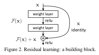
According to ResNet, we should have two weight layers, an identity (skip-connection) block and activation (ReLU), which is exactly ResBlock implements, with many tweaks introduced in the following years to improve the performance. A ConvLayer in fastai is Conv2D --> BatchNorm --> activation (ReLU). For the other variants of xresnet, we'll have exact same architecture but with more "groups" of ResBlock, such as

def xresnet34 (pretrained=False, **kwargs): return _xresnet(pretrained, 1, [3, 4,  6, 3], **kwargs)
def xresnet50 (pretrained=False, **kwargs): return _xresnet(pretrained, 4, [3, 4,  6, 3], **kwargs)
def xresnet101(pretrained=False, **kwargs): return _xresnet(pretrained, 4, [3, 4, 23, 3], **kwargs)
def xresnet152(pretrained=False, **kwargs): return _xresnet(pretrained, 4, [3, 8, 36, 3], **kwargs)

xresnet34 will have 4 groups having [3, 4, 6, 3] no. of ResBlocks and so on. We do get other variants of these base architecutures but as they're still experimental, I'll skip them for now. Now let's have a look at some architectures from torchvision.

MNasNet (torchvision)

from torchvision.models import MNASNet
mnasnet = MNASNet(1.0)

First 7 layers are stem of the network while 8 to 13 seems like some specific blocks of this architecture.

arch_summary(mnasnet,0)
[0 ] Conv2d           : 1   layers
[1 ] BatchNorm2d      : 1   layers
[2 ] ReLU             : 1   layers
[3 ] Conv2d           : 1   layers
[4 ] BatchNorm2d      : 1   layers
[5 ] ReLU             : 1   layers
[6 ] Conv2d           : 1   layers
[7 ] BatchNorm2d      : 1   layers
[8 ] Sequential       : 3   layers
[9 ] Sequential       : 3   layers
[10] Sequential       : 3   layers
[11] Sequential       : 2   layers
[12] Sequential       : 4   layers
[13] Sequential       : 1   layers
[14] Conv2d           : 1   layers
[15] BatchNorm2d      : 1   layers
[16] ReLU             : 1   layers
arch_summary(mnasnet,[0,8])
[0 ] _InvertedResidual: 8   layers
[1 ] _InvertedResidual: 8   layers
[2 ] _InvertedResidual: 8   layers

Yup, they're InvertedResidual blocks. Let's find out what is InvertedResidualBlock

get_module(mnasnet,[0,8,0])
_InvertedResidual(
  (layers): Sequential(
    (0): Conv2d(16, 48, kernel_size=(1, 1), stride=(1, 1), bias=False)
    (1): BatchNorm2d(48, eps=1e-05, momentum=0.00029999999999996696, affine=True, track_running_stats=True)
    (2): ReLU(inplace=True)
    (3): Conv2d(48, 48, kernel_size=(3, 3), stride=(2, 2), padding=(1, 1), groups=48, bias=False)
    (4): BatchNorm2d(48, eps=1e-05, momentum=0.00029999999999996696, affine=True, track_running_stats=True)
    (5): ReLU(inplace=True)
    (6): Conv2d(48, 24, kernel_size=(1, 1), stride=(1, 1), bias=False)
    (7): BatchNorm2d(24, eps=1e-05, momentum=0.00029999999999996696, affine=True, track_running_stats=True)
  )
)

Inverted Residual

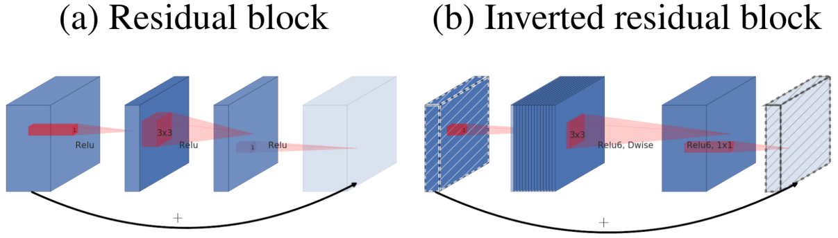
If you spot the difference, Residual Blocks have a fat input block being shrunk down before performing actual 3 × 3 convolution whereas inverted residuals have exact opposite picture.

A compact input block is first expanded, the convolution op is performed and again that block is compressed back to a compact version.

WideResnet

from torchvision.models import wide_resnet50_2
arch_summary(wide_resnet50_2)
[0 ] (conv1)    Conv2d           : 1   layers
[1 ] (bn1)      BatchNorm2d      : 1   layers
[2 ] (relu)     ReLU             : 1   layers
[3 ] (maxpool)  MaxPool2d        : 1   layers
[4 ] (layer1)   Sequential       : 3   layers
[5 ] (layer2)   Sequential       : 4   layers
[6 ] (layer3)   Sequential       : 6   layers
[7 ] (layer4)   Sequential       : 3   layers
[8 ] (avgpool)  AdaptiveAvgPool2d: 1   layers
[9 ] (fc)       Linear           : 1   layers

If you look at the sequential layers, they do have no. of children exact similar to resnet50, while the key difference here is no. of input and output channels of their special block. Let's figure out what it is

arch_summary(wide_resnet50_2,[4])
[0 ] Bottleneck       : 9   layers
[1 ] Bottleneck       : 7   layers
[2 ] Bottleneck       : 7   layers

You can also use the module names listed above to get required module, but you might need to take care of instantiating an object

arch_summary(wide_resnet50_2().layer1)
[0 ] Bottleneck       : 9   layers
[1 ] Bottleneck       : 7   layers
[2 ] Bottleneck       : 7   layers

As discussed earlier, we'll be using get_module to find exact definition of Bottleneck block

get_module(wide_resnet50_2,[4,0])
Bottleneck(
  (conv1): Conv2d(64, 128, kernel_size=(1, 1), stride=(1, 1), bias=False)
  (bn1): BatchNorm2d(128, eps=1e-05, momentum=0.1, affine=True, track_running_stats=True)
  (conv2): Conv2d(128, 128, kernel_size=(3, 3), stride=(1, 1), padding=(1, 1), bias=False)
  (bn2): BatchNorm2d(128, eps=1e-05, momentum=0.1, affine=True, track_running_stats=True)
  (conv3): Conv2d(128, 256, kernel_size=(1, 1), stride=(1, 1), bias=False)
  (bn3): BatchNorm2d(256, eps=1e-05, momentum=0.1, affine=True, track_running_stats=True)
  (relu): ReLU(inplace=True)
  (downsample): Sequential(
    (0): Conv2d(64, 256, kernel_size=(1, 1), stride=(1, 1), bias=False)
    (1): BatchNorm2d(256, eps=1e-05, momentum=0.1, affine=True, track_running_stats=True)
  )
)

Let's compare it with original resnet50. The idea proposed by WideResnet was having more channels in the bottleneck layers to exploit the parallelism offered by GPUs. Thus wideresnets take lesser time to train and to reach the error rate achieved by resnets.

get_module(resnet50,[4,0])
Bottleneck(
  (conv1): Conv2d(64, 64, kernel_size=(1, 1), stride=(1, 1), bias=False)
  (bn1): BatchNorm2d(64, eps=1e-05, momentum=0.1, affine=True, track_running_stats=True)
  (conv2): Conv2d(64, 64, kernel_size=(3, 3), stride=(1, 1), padding=(1, 1), bias=False)
  (bn2): BatchNorm2d(64, eps=1e-05, momentum=0.1, affine=True, track_running_stats=True)
  (conv3): Conv2d(64, 256, kernel_size=(1, 1), stride=(1, 1), bias=False)
  (bn3): BatchNorm2d(256, eps=1e-05, momentum=0.1, affine=True, track_running_stats=True)
  (relu): ReLU(inplace=True)
  (downsample): Sequential(
    (0): Conv2d(64, 256, kernel_size=(1, 1), stride=(1, 1), bias=False)
    (1): BatchNorm2d(256, eps=1e-05, momentum=0.1, affine=True, track_running_stats=True)
  )
)